
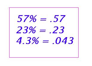
z scores
percentages and z scores
percentages above or below some raw score
percentages between two raw scores
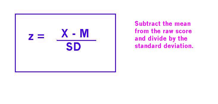
Use the z score formulas in your Horror book. In general,
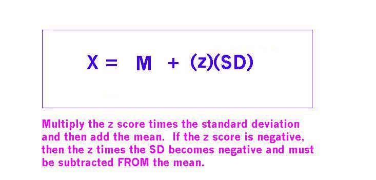
If your problem asks you to find a raw score, you need to use the transformation of the z formula that starts out with X =.
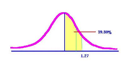
This means that 39.80 percent of the entire
normal curve is found between
the mean and the z score of 1.27.
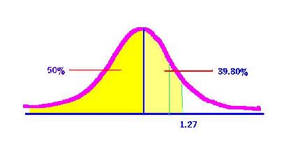
Now, if we wanted to know how much of the normal curve was located below the z score of 1.27, we would have to add the 39.8 percent to the 50 percent located below the mean.
The percentile for a z score of 1.27 is 89.8.
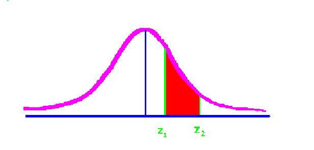
For this problem, you want to know what is the percent of the curve falling below the raw score of 9 hours.
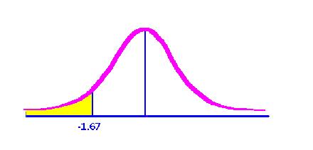
First, determine the z score at 9 hours. The mean is 14 and the standard deviation is three. The z would be 9 minus 14, divided by 3, or -1.67. So, now you are getting closer to knowing what percent of eggs could be thrown at the end of just 9 hours. That would be the amount of time you'd have to spend doing just one of these problems, right?
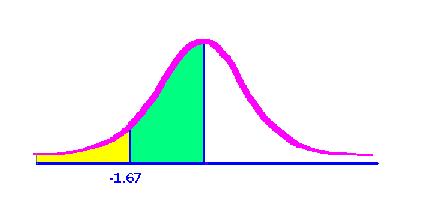
Now go to page 523 to find the area between the mean and -1.67. That percent is 45.25. So the green area, estimated by the curve to the right, is 45.25%. The yellow area, then, must be 50% minus 45.25%, or 4.74%. Therefore, however many eggs you had to begin with, you'd be able to throw 4.74% of them at your stats professor.
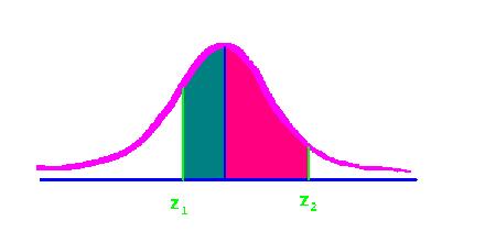
Yes, find the area between each z score and the mean and ADD them together. Here's an example: Suppose you wanted to find the percentage between the two raw scores of 45 and 57 for a distribution with a mean of 50 and a standard deviation of 3.
The z score for 45 is (45 - 50)/3, or -1.67. The z score for the 57 is (57 - 50)/3, or 2.33. The first z is on the left side of the mean and the second is on the right side of the mean. The percentage for the -1.67 is 45.25. The percentage for the 2.33 is 49.01. Together, the percentage is 94.26. Therefore,94.26 percent of the population resides between those two raw scores, given the mean of 50 and the SD of 3.
Suppose the first z score were .69. The percent between the mean and the z of .69 is 25.49. If the second z score were 1.73 then the percent (in blue below) would be 45.82.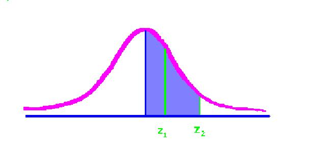
(12 - 9.5)/ 3.15 = .79
Look that up in the z table and you'll find that the percentage between the mean and .79 is 28.52%.
The problem asks us to find the probability of MORE than 12 cavities so we'd need to subtract 28.52 from 50% to get what's on the other side. The percentage is 21.48.
Now, all you need to do to find the PROBABILITY is to change 21.48% to its decimal form, or .2148.
Therefore, p = .215 (round however you like). Not too bad, no? Chapter Six problems are just like those in
Chapter 4. The only difference is that once you have found the percentage, you then change it to a decimal (a probability). To change a percent to a probability, take off the percent sign and move the decimal two places to the left. You are, in essence, dividing the numeral by 100. Afterall, percent means per hundred, or, divide by 100.
Let's work problem 11 in Chapter 6: You know the mean is 9.5 and the standard deviation is 3.15. To find the probability of finding at random someone who had more than 12 filled cavities, you assume that 12 is the X (score).
Use the z formula to find out how far (in standard deviations) from the mean the 12 is.
Back to Week Two
Back to Statistics Helps
Home
This page is intended to help you with the third week's materials. You should be feeling just a little better.
z test
distributions
single sample t test
independent t test
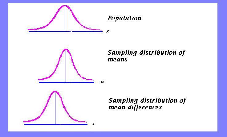
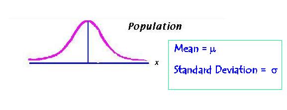
The first one is a population of raw scores. It has a mean, mu and a standard deviation, sigma.
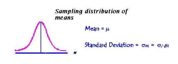
The second is the distribution of means. It is called a sampling distribution because it assumes that many samples of a particular size have been randomly drawn from the population. The means from all those samples then form a distribution. The distribution is also normal in shape, provided the population was normal. The mean for the distribution of means is the same as the original population, mu, and the standard deviation of the means is sigma divided by the square root of the sample size. The standard deviation of the means is called the standard error of the means.
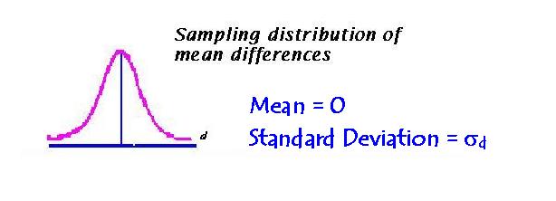
The third distribution is also a sampling distribution. It is the distribution of mean differences. It is based on the assumption that two random samples are taken from the same distribution, and their difference is found. This is done many times until a distribution of mean differences is formed. If you think about it, the mean would be at that spot where the two sample means were the same. If we subtract a mean from itself, we would get zero, so... the mean of the distribution of differences is zero. The standard deviation of this distribution is,... you guessed it -- the standard deviation of differences. It is called the standard error of difference.
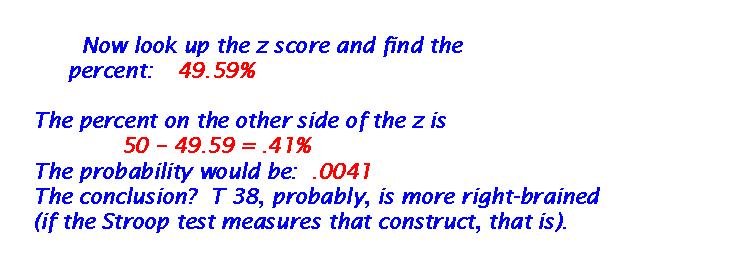
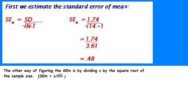
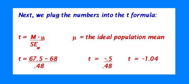
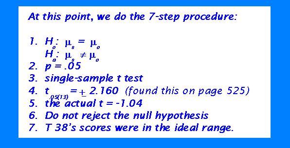
Suppose we wanted to see if the T 38 scores on the final were ideal. Let's set the ideal at 68 out of 75 points. This will involve a two-tailed hypothesis: ideal or not. Suppose the mean for T 38 is 67.5, with a standard deviation of 1.74 points. Did T 38 score optimally?
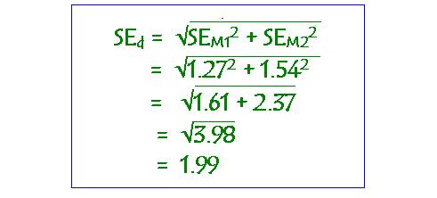
Suppose we'd like to know if SNU students do better on the stat final than do, say, OU students. Suppose a random sample of 26 stat students is taken from each school and given the Horror Stat Exam. Suppose that SNU's mean is 69.3, with a standard deviation of 6.35. Suppose that OU's mean is 63.4, with a standard deviation of 7.7. The standard error of the mean for SNU would be 6.35 divided by the square root of 25, or 1.27. OU's standard error of the mean would be 7.7 divided by the square root of 25, or 1.54. Next, the standard error of difference would need to be determined.
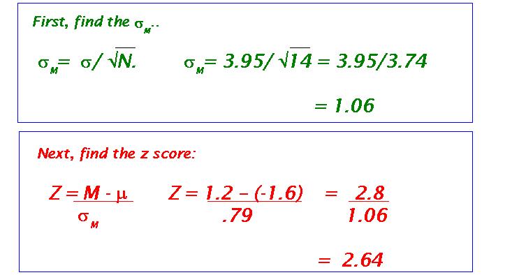
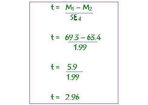
Now, we need to plug in the figures in the t formula.
Now let's do the 7 step procedure. Let's assume that we expected a direction -- yes, we expected that SNU would do better than OU.
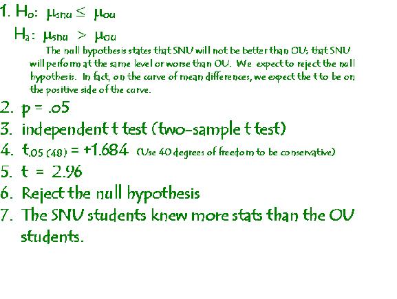
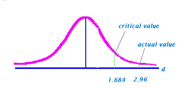
Note where the actual t falls in relation to the critical value.